Month: August 2014

Creating and Reading XML files with Python

A few days ago my mentor gave me the task of reading an XML file and then creating a new XML file in a different format by using the data of the read XML file. Since I was given the full freedom of using any programming language, I decided to go with C as taking CS50x has now given me enough confidence to approach any programming dragon with my shining C sword and armor. However after a few hours, I realized that I was getting nowhere. So I decided to look into Python. It turns out that working with XML files is an extremely simple task using Python.

For my task I made use of the ‘xml.etree’ and ‘xml.minidom’.

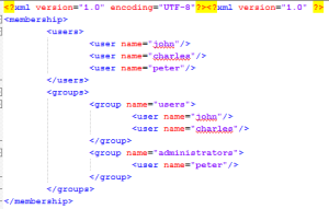
I will now give you a step by step guide on how to create a beautiful (pretty-print) XML file as shown below using python and also some tips on how to read an XML file.

xml

Step 1: Importing the libraries.

import xml.dom.minidom
from xml.etree import ElementTree
from xml.etree.ElementTree import Element
from xml.etree.ElementTree import SubElement

Step 2: Creating the root element.

# <membership/>
membership = Element( 'membership' )

Step 3: Creating child for the root. I will create two children for the root in this example.

# <membership><users/>
users = SubElement( membership, 'users' )
# <membership><groups/>
groups = SubElement( membership, 'groups' )

Step 4: Creating nodes inside the children.

# <membership><users><user/>
SubElement( users, 'user', name='john' )
SubElement( users, 'user', name='charles' )
SubElement( users, 'user', name='peter' )
# <membership><groups><group><user/>
SubElement( group, 'user', name='john' )
SubElement( group, 'user', name='charles' )
# <membership><groups><group/>
group = SubElement( groups, 'group', name='administrators' )
# <membership><groups><group><user/>
SubElement( group, 'user', name='peter' )

Step 5: Converting to string and then pretty-print.

xmls = xml.dom.minidom.parseString(string)
pretty_xml_as_string = xmls.toprettyxml()

Step 6: Writing to a file.

output_file = open('membership.xml', 'w')
output_file.write('')
output_file.write(pretty_xml_as_string)
output_file.close()

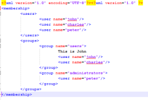
This will create a nice XML file for us. If you want to add a text node also just use the following command:
group.text = "This is John"
after any of the element or sub-element which is assigned to users, and it will ad a text-node to the file like below.

text_node

While reading an XML file we must proceed in an hierarchical manner.

from xml.etree import ElementTree
document = ElementTree.parse( 'membership.xml' )

document will have an object that is not exactly a node in the XML structure, but it provides a handful of functions to consume the contents of the element hierarchy parsed from the file. Which way you choose is largely a matter of taste and probably influenced by the task at hand. The following are examples:

users = document.find( 'users')

is equivalent to:

membership = document.getroot()
users = membership.find( 'users' )


Finding specific elements

XML is a hierarchical structure. Depending on what you do, you may want to enforce certain hierarchy of elements when consuming the contents of the file. For example, we know that the membership.xml file expects users to be defined like membership -> users -> user. You can quickly get all the user nodes by doing this:

for user in document.findall( 'users/user' ):
print user.attrib[ 'name' ]

Likewise, you can quickly get all the groups by doing this:

for group in document.findall( 'groups/group' ):
print group.attrib[ 'name' ]

Iterating elements

Even after finding specific elements or entry points in the hierarchy, you will normally need to iterate the children of a given node. This can be done like this:

for group in document.findall( 'groups/group' ):
print 'Group:', group.attrib[ 'name' ]
print 'Users:'
for node in group.getchildren():
if node.tag == 'user':
print '-', node.attrib[ 'name' ]

Other times, you may need to visit every single element in the hierarchy from any given starting point. There are two ways of doing it, one includes the starting element in the iteration, the other only its children. Subtle, but important difference, i.e.:

Iterate nodes including starting point:

users = document.find( 'users' )
for node in users.getiterator():
print node.tag, node.attrib, node.text, node.tail

Produces this output:

users {} None None
user {'name': 'john'} None None
user {'name': 'charles'} None None
user {'name': 'peter'} None None
Iterate only the children:

users = document.find( 'users' )
for node in users.getchildren():
print node.tag, node.attrib, node.text, node.tail

Produces this output:

user {'name': 'john'} None None
user {'name': 'charles'} None None
user {'name': 'peter'} None None
 

I am now a forensic expert !

Okay, so the title is a bit of an exaggeration, but still the task that I managed to do today was something that I had never believed in my wildest dreams that I would be able to accomplish. I just learnt how to recover deleted files using just about hundred lines of C code. Yes! you heard (or rather read) it right. All this was made possible due to the amazing CS50x MOOC that I am taking on edX, an online learning platform.

CS50x is the edX version of the popular CS50 course of the Harvard University, taught by Prof. David J. Malan who is an exceptionally great teacher and one of the best instructor that I have ever had the pleasure of learning from. So as part of the 5th Problem Set (more on first five later), we (who we? the people who are taking the course, duh!) were required to retrieve about 50 jpeg images, which had supposedly been deleted “by mistake”. To solve this problem, some basic knowledge of the JPEG file format, FAT file system and how the images are stored in a CompactFlash (CF) card are stored is required.

So we all know (well at least most of us) that an image is nothing but a large number of pixel values that are stored in some specific order with a specific format. It turns out that the JPEGs too have patterns of bytes that distinguish them from other file formats. In fact, most JPEGs begin with one of two sequences of bytes. Specifically, the first four bytes of most JPEGs are either

0xff 0xd8 0xff 0xe0

or

0xff 0xd8 0xff 0xe1

from first byte to fourth byte, left to right. Odds are, if you find one of these patterns of bytes on a disk known to store photos then that means that they de-mark the start of a JPEG.

Also it turns out that when you delete a file in a FAT file system, it is not actually erased from memory. What actually happens is that  the system modifies the filename’s first character in the file’s directory entry to signal that the file has been deleted and that the directory entry can be recycled. Second, the system moves all of the file’s FAT clusters to the hard drive’s list of free clusters. Thus, as you might guess, we can easily recover any deleted files by scavenging through the file-system for some specific byte pattern.

You can read more about it from here : http://d2o9nyf4hwsci4.cloudfront.net/2013/fall/psets/5/garfinkel.pdf

Furthermore, digital cameras tend to store photographs contiguously on CF cards, whereby each photo is stored immediately after the previously taken photo. Accordingly, the start of a JPEG usually demarks the end of another. However, digital cameras generally initialize CF cards with a FAT file system whose “block size” is 512 bytes (B). The implication is that these cameras only write to those cards in units of 512 B. A photo that’s 1 MB (i.e., 1,048,576 B) thus takes up 1048576 ÷ 512 = 2048 “blocks” on a CF card. But so does a photo that’s, say, one byte smaller (i.e., 1,048,575 B)! The wasted space on disk is called “slack space.” Forensic investigators often look at slack space for remnants of suspicious data.

So now lets come to our problem. According to the problem statement, we must read a *.raw format file, which is nothing but a “forensic image” of the card and store its contents, byte after byte. We just open the file using the  fopen(…) function and then read through it using the fread(…) function. Also we read in 512 bytes into the buffer at a time (because a block is stored as 512 bytes in FAT file-system) and then check if the starting 4 bytes represent the start of a JPEG file. If they do, then we have found an image and we write all the block’s data into a file using fwrite(…), and continue writing the next blocks into the same file until we encounter another block which starts with JPEG specific 4 byte format. Since our CF card stores images contiguously as mentioned earlier, we  need not worry about random files and garbage values coming in the middle of two blocks. When we find a another pattern that signifies an new jpeg image, we close our present file and create a new file with a new name, and start writing the data into it until we encounter another JPEG start specific byte pattern.

Continuing this way, we will reach the end of the file, at which point we must close our input *.raw file and our newly written *.jpeg file.

If you do everything right (as I did :P), you will hopefully end up recovering your deleted images. Does’nt it sound too easy? Well, it actually is. It took me less than two hours to go through the entire problem statement for the Forensics assignment and complete it. Also it was the most interesting piece if code that I had ever written (I am not a Computer Science student, and no I don’t code all day). And having done that, I am now going to insert my camera memory card into my computer, delete all the images and then hopefully recover them successfully. So have fun trying this yourself and as they say, “This is CS50”.


#3 Linear Regression with Multiple Variables

In the previous post I talked about the simple case in which we were able to fit our data-set with the help of only one variable. But life is not so simple. In most of the real-life scenarios the data-set will have more than one feature, i.e the output may be dependent on more than one variable. Taking the case of the previous example of housing prices, the price of the house may not only depend on the size of the house but also on the say, the age of the house, the number of rooms in the house, etc. In such cases using the simple linear regression (h = to + t*x) may not work.

Rather we must formulate a new equation which takes care of all the parameters. Turns out this is also quite simple. So suppose you have a data-set in which there are say 4 features. We can then model it using the equation:

h = to+ x1*t1+ x2*t2+ x3*t3+ x4*t4                                                                        equation 1

where x1 is the value of feature 1 (say age of the house), x2 is the value of the second feature (say number of rooms in the house) and so on.

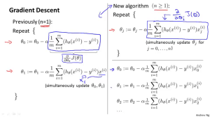
So now our hypothesis (h) is an (n+1) dimensional vector if there are n features in the training set. The cost function remains the same (J = 1/2m * [sum(h(i) – y(i)]^2  over all points) with h calculated using equation 1. To optimize it we may use our loyal gradient descent algorithm with only a slight modification. Shown below are the equations taken directly from the lecture slides (by Prof. Andrew Ng of Stanford University)

mutivar_gd

What we are simply doing for this case is updating the values for all the parameters simultaneously.

Now as you might guess, this process will become computationally a little expensive if we have a large data-set with a lot of features. In such cases usually there are two ways to speed up the process: 1) Feature Scaling using Mean Normalization; 2) Varying the learning rate.

1) Feature Scaling using Mean Normalization simply means hat we replace each parameter (x1, x2, …) with (x(i) – mean(i))/range, where x(i) is the ith parameter, mean(i) is the mean of the ith feature column and range is simply the standard deviation or max-min value of that feature column.

2) Varying learning rate implies increasing the value of alpha in the above equation. As stated in my last post, if alpha is too small, the algorithm may take a lot of time to converge, while if alpha becomes too high, the Cost function may begin to diverge. So an optimum value of alpha must be chosen by trial and error.


Now Gradient Descent is not the only algorithm that can help us optimize our cost function (J). As Prof. Andrew mentioned, Normal Regression is another great way to optimize our cost function. In this method we neither have have to choose alpha nor iterate over multiple steps. This method gives the optimum point in one step. However it is not suitable if number of features is very large because it might be very slow. In such cases gradient descent works well even with large number of features. Since this is a slightly complex algorithm with a lot of matrix notations, I will not discuss it here for fear of my post becoming too large and complex. But if it really interests you, then please go through the Week 2 lecture videos 6 and 7. However for most of our cases, the gradient descent works just fine.

In the next post I will talk about Logistic Regression and Classification.

Stay tuned….